Meningioma Classification using Machine Learning
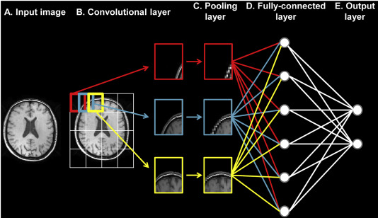 PC: Basaia, Silvia, et al. NeuroImage: Clinical 21 (2019)
Problem Statement
Meningiomas are tumors that form on the meninges, a membrane that covers the brain and spinal cord. The current standard of treatment is a craniotomy where the skull is opened to provide access to the tumor. Recent technological advances have allowed meningioma’s to be resected using minimally invasive endoscopic or key-hole surgical approaches.1 The selection of patients for these minimally invasive surgeries are based on several tumor characteristics such as pathology, vascularity, and invasiveness.1
One key characteristic that dictates ease of operation is tumor consistency, defined as texture or firmness.1 Tumor consistency, which can only be measured after surgical resection, is graded on a 5-point hardness scale (1-softest, 5-hardest).1,2 Training a machine learning model to classify a tumor according to its hardness using neuroimaging data could help physicians determine if a patient is a candidate for minimally invasive surgery.
Objective
To train a convolutional neural network to classify meningioma tumors based on hardness ratings.
Code can be downloaded at: https://github.com/arsakhar/ML-Meningioma-Classification
Data Acquisition
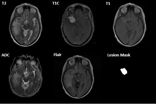
MRI scans were acquired on 85 patients across several hospitals. For each patient, an ADC, T2 flair, T1, T1 with contrast (T1c), and T2 scan were acquired. A lesion mask was manually created by the physician after image acquisition. Resected meningioma’s were manually labeled using a 0-3 hardness scale by expert raters.
Pre-Processing
A supervised learning task for multi-class classification was considered based on the provided labels and discrete grading scale. A convolutional neural network classifier was chosen as the inputs were images.
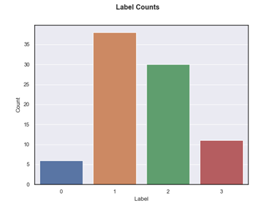
The bar chart below shows the distribution of meningioma classes for the acquired data. Class 0 and 1 were the lowest and highest frequency, respectively. Overall, the dataset was highly imbalanced between classes 1, 3 and 1,2. Moreover, only a limited sample of 425 scans (85 patients and 5 scans per patient) were available for training the model.
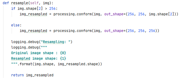
One issue with the acquired data was that the dimensions of the scans were consistent within a subject but differed between subjects. Briefly, an MRI scan is a 3D volume of height, width, and depth where depth represents the number of slices.
To ensure a consistent input shape into the CNN, each scan was resampled to a size of 256x256xZ. Z was set to 256 if the image had less than 256 slices. Otherwise, the original number of slices was retained.
To increase the number of available training samples, each scan was decomposed into its individual slices.
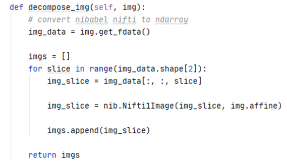
The figure below illustrates multiple slices across a single scan.
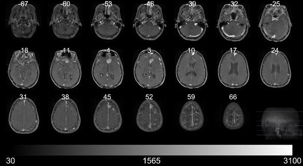
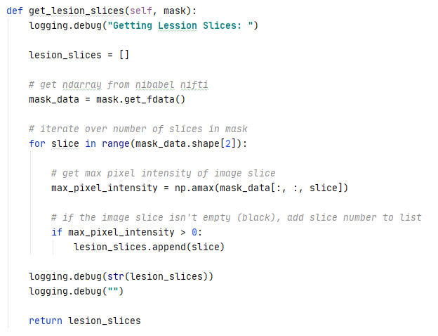
Each individual slice was then re-assigned the original class label only if it contained the lesion based on the lesion mask. Slices that did not contain a lesion were not included in training the model. Decomposing and re-assigning class labels increased the accuracy of the label assignments as a single label was no longer applied to an entire 3D volume.
Training
Residual Neural Network 152 (ResNet 152) was selected as the CNN model for training. The following hyperparameters were randomly selected and evaluated using Optuna:
- Optimizer – Adam, RMSprop, SGD
- Learning Rate – log uniform distribution, [1e-6, 1e-1]
- Dropout – uniform distribution, [0.1, 0.7]
- Batch Size – categorical, [16, 32, 64, 128]
- L2 Regularization – log uniform distribution, [1e-10, 1e-3]
The remaining training parameters were set as follows:
- Input Channels – 5 [t1, t1c, t2 flair, t2, adc]
- # Classes – 4
- # Epochs – 45
- Loss function – cross-entropy
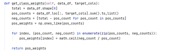
The cross-entropy loss function was weighted according to the distribution of classes in the dataset.
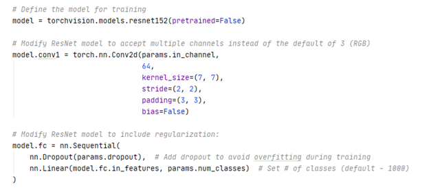
Two modifications were made to the original ResNet152 model. The first convolutional layer was modified to accept 5 input channels instead of 3 and the fully connected layer was modified to output probabilities for 4 classes instead of 1000.
The ResNet 152 model was trained using 5-fold cross validation. The folds were stratified by subject to ensure all slices associated with a single subject were constrained to a single fold. Briefly, neighboring slices within a scan are structurally similar as they are anatomically acquired a few mm apart. This problem is exacerbated in subjects where the scan is up sampled to 256 slices during preprocessing. The similarity of slices results in data leakage if the slices are spread across the training and test fold. The folds were also stratified by class label to ensure the distribution of classes in the training and test fold approximated the actual distribution of classes for the acquired data.
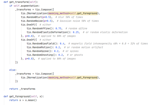
A custom dataset class was used to load, augment, and transform the slices to tensors for input into the CNN. TorchIO, a python package for medical image preprocessing, was used for data augmentation. Briefly, both training and validation slices were normalized to a mean of zero and standard deviation of one. Training slices were also augmented with a random blur, noise, bias field, motion, spike, ghosting, affine transformations, and elastic deformations at specified probabilities. This was done to provide additional unique images for the CNN to train on in the absence of a large training dataset.
Each epoch consisted of a training and validation iteration. Both iterations consisted of a forward pass. Loss was calculated using the SoftMax output and target labels. The weights and bias in each layer were updated via back propagation for the training iterations. The argmax of the SoftMax output probabilities was used to calculate accuracy, defined by the proportion of correct predictions to total predictions.
Results
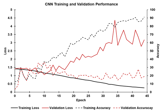
Overall, the trained CNN model performed poorly on the validation dataset across multiple sets of hyperparameters selected by Optuna. The figure below shows the training and validation loss accuracy for a single fold and set of hyperparameters. As expected for training, the loss decreased (solid black line) and accuracy (dashed black line) increased, with accuracy approaching 95% after 45 epochs. However, validation loss (solid red line) and validation accuracy (dashed red line) did not improve during training. Validation loss decreased for the first 10 epochs before increasing. The validation accuracy increased to approximately 35% after 10 epochs before decreasing to 20%. Therefore, overfitting likely occurred after the 10th epoch.
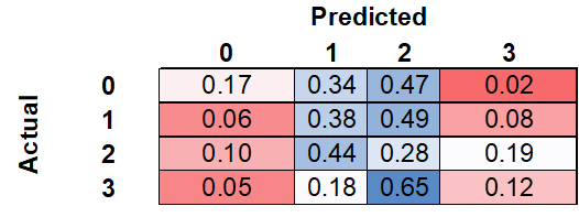
The confusion matrix, calculated as a normalized sum of the confusion matrices for each k-fold, can be seen below. Of the meningiomas with an actual label of zero, the model correctly labeled 17%, while incorrectly labeling 34% and 47% as one and two, respectively. Of the meningiomas with an actual label of three, the model correctly labeled 12%, while incorrectly labeling 18% and 65% as one and two, respectively.
Discussion
Overall, the CNN was unable to classify Meningioma’s with high accuracy and generalized very poorly to unseen validation data. The highest validation accuracy across the training folds was only 35% which is marginally better than 25% due to random guessing. The poor validation accuracy was seen for multiple combinations of hyperparameters decreasing the likelihood that the results were due to a poorly optimized model.
Poor model performance may be due a lack of discernible patterns between classes of meningioma observed on an MRI. Indeed, it is possible that the biological properties underlying the tactile hardness, texture, and consistency differences observed by the expert rater during grading are not detectable on an MRI. It is also possible that inter-rater and intra-rater variability resulted in misclassification of some meningioma’s during labeling. This variability could affect model training as the labels are not representative of the actual ground truth.
Despite the poor overall accuracy, the model was able to discriminate between the extreme classes, zero and three, relatively well. As seen in the confusion matrix, the model rarely assigned class three to class zero and vice versa. Taken together, this suggests that there may be a detectable pattern between classes.
Future Directions
Due to computational requirements, the grid search for the optimal hyperparameters was only run for 3 iterations. Furthermore, only the ResNet 152 CNN was trained. Training additional CNN’s and continuing the grid search over 10-15 iterations may yield a trained model better suited for the provided dataset. Different data augmentation techniques may also improve model training as well. However, these changes will likely only result in a marginal improvement in classification accuracy. To evaluate whether Meningioma’s acquired by MRI can be classified with high accuracy, additional training data is needed.
In the absence of additional training data, one possibility is to run an unsupervised machine learning technique such as k-means clustering over a range of clusters. A scree plot or silhouette analysis can then be used to identify the optimal number of clusters. The labels of the images in each cluster can then be compared to identify the purity of the cluster. If the optimal number of clusters is 4, it would suggest there is a detectable pattern aligned with the expected number of classes. Moreover, if the incorrectly labeled images in each cluster are better suited for the nearest neighboring cluster. it may suggest that inter-rater and intra-rater variability are contributing to problems with model training.
References
- Shiroishi, Mark S., et al. “Predicting meningioma consistency on preoperative neuroimaging studies.” Neurosurgery Clinics 27.2 (2016): 145-154.
- Zada, Gabriel, et al. “A proposed grading system for standardizing tumor consistency of intracranial meningiomas.” Neurosurgical focus 35.6 (2013): E1.
Technical Skills
- Pre-processing MRI data
- Manipulating and training a convolutional neural network for image classification
- Cross-validation for small datasets
- Generating classification reports and confusion matrices
Packages
- Optuna
- NiBabel
- Pandas
- NumPy
- Torch
- Torchvision
- Scikit-learn
- TorchIO